The Fundamental Distinction Between Ordinal and Interval Scales in Quantitative Data Analysis

Human cognition is inherently driven by the desire to organize the chaotic nature of the world into neat, sequential hierarchies. From the collegiate rankings that dictate admissions strategies for millions of families to the performance scorecards that influence corporate compensation, the impulse to rank is omnipresent. However, a growing body of research in data science and statistical methodology suggests that society often conflates two distinct modes of measurement: ordinal scaling and interval scaling. This confusion leads to significant errors in analytical reasoning, particularly in fields as diverse as social science research, human resources, and market analytics.

The Anatomy of Ordinal Scaling

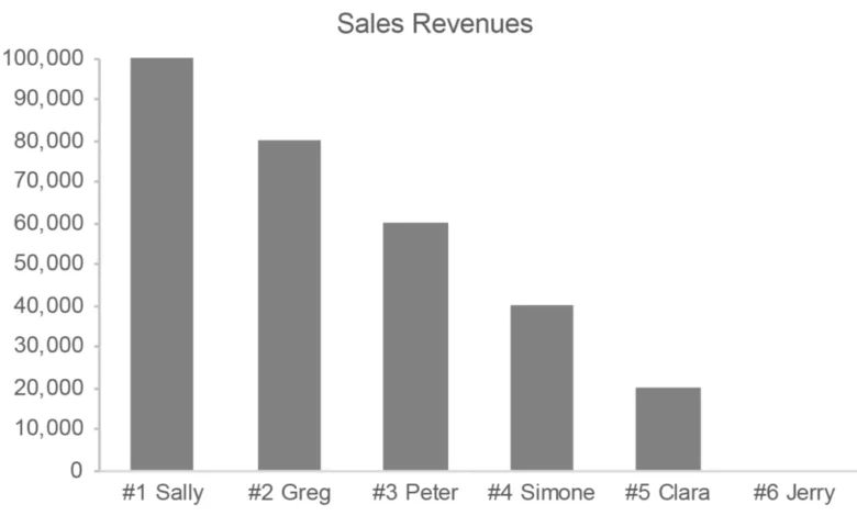
An ordinal scale is defined by its ability to represent a meaningful order of items without providing information regarding the magnitude of the differences between those items. For instance, if a sales team is ranked from first to fourth, the list communicates a sequence of performance. However, it fails to quantify the actual output. The gap between the first-place salesperson and the second-place individual may represent a million-dollar difference in revenue, while the gap between the second and third might be a mere few hundred dollars. In this scenario, the ordinal ranking is a tool for relative placement, not a tool for calculating productivity.

The historical application of ordinal scales dates back to early psychological research. In the late 19th and early 20th centuries, as social scientists sought to quantify subjective human experiences—such as happiness, anxiety, or political inclination—they struggled with the lack of a universal unit of measurement. The invention of the Likert scale, named after psychologist Rensis Likert, provided a structured response format to capture these qualitative sentiments. By providing respondents with a range from "Never" to "Always," researchers could organize responses linearly.

However, a critical failure often occurs when researchers treat these five-point or seven-point scales as if they were ratio data. If a survey asks a respondent to rate their satisfaction from 1 to 5, the difference between "1" and "2" is not mathematically guaranteed to be identical to the difference between "4" and "5." By treating these labels as quantitative values, researchers risk creating a false sense of precision, a practice that frequently leads to flawed conclusions in academic and commercial reporting.

Understanding Interval Scales: The Quantitative Standard

In contrast to the ordinal model, an interval scale provides a consistent measurement where the distance between each point is uniform. A common example is a timeline of fiscal years. The distance between 1950 and 1960 is exactly ten years, identical to the distance between 2000 and 2010. In this structure, the data points possess a quantitative nature that allows for rigorous arithmetic manipulation.

In data visualization, the distinction between these two scales is vital. When graphing data, the choice of scale dictates the viewer’s perception of the underlying reality. If a graph displays salespeople using an ordinal rank, the viewer may mistakenly perceive the performance gaps to be equal across the board. If the data is instead represented using an interval scale—such as a bar chart reflecting raw revenue—the viewer immediately gains an accurate understanding of the performance variance.

Historical Context and the Evolution of Measurement

The need for strict differentiation between these measurement types became particularly acute during the mid-20th century, a period marked by the "Quantification Movement." As computing power increased, the ability to collect large datasets grew, and organizations became eager to convert every possible observation into a number. During the 1960s and 1970s, the rise of the "Customer Satisfaction Index" (CSI) across various industries saw a proliferation of Likert-based surveys.

The timeline of this methodological evolution follows a clear trajectory:

• 1932: Rensis Likert publishes his thesis, introducing the Likert scale as a method for measuring attitudes.
• 1946: Psychologist Stanley Smith Stevens publishes his landmark paper "On the Theory of Scales of Measurement" in Science, where he explicitly defines nominal, ordinal, interval, and ratio scales. This paper remains the bedrock of modern psychometrics.
• 1970s-1990s: The widespread adoption of computer-aided telephone interviewing (CATI) leads to a massive increase in survey data, much of which relies on ordinal scoring systems.
• 2000s-Present: Data scientists begin to push back against the "ordinal-as-quantitative" fallacy, as high-stakes machine learning models and predictive analytics demand higher data fidelity.

Supporting Data: The Risk of Misinterpretation

Evidence of the risks inherent in misusing ordinal data can be found in performance management metrics. In a study of corporate sales departments, researchers found that when sales managers relied exclusively on ordinal rankings rather than raw output, they were 30% more likely to misallocate resources, such as bonuses and training time. Because ordinal scales mask the magnitude of the "top-performer effect," managers often failed to identify the true outliers in their teams.

Furthermore, in public health research, the use of Likert scales to measure clinical depression—where researchers aggregate scores into a total—has been widely criticized. By adding up points from subjective questions, the final result provides an illusion of a clinical score. Critics, such as those at the Perceptual Edge research group, argue that this practice generates "pseudo-quantitative" data that lacks the stability required for diagnostic accuracy.

Official Responses and Academic Consensus

The consensus among statisticians is increasingly clear: ordinal data should be analyzed using non-parametric statistics, while interval data can support more robust parametric testing. Organizations such as the American Statistical Association (ASA) have issued guidelines cautioning against the aggregation of Likert-type data for the purpose of creating "averages."

"The primary error," writes one analyst in a peer-reviewed review of survey methodology, "is the assumption that the linguistic labels assigned to numbers—such as ‘agree’ or ‘strongly agree’—are equidistant. There is no empirical evidence to support that a respondent’s move from ‘agree’ to ‘strongly agree’ is the same cognitive leap as moving from ‘neutral’ to ‘agree.’"

Broader Impact and Implications

The implications of failing to distinguish between these scales extend into the realms of public policy and economic forecasting. When governments or central banks rely on "sentiment surveys" that quantify consumer confidence through ordinal-to-quantitative conversion, they are effectively building policy on a foundation of sand. If the measurement tool is flawed, the resulting economic model is inherently biased.

For data professionals, the takeaway is to maintain rigorous separation between how data is presented and how it is analyzed. In visualization, this means using dot plots or bar charts that reflect raw values whenever possible, rather than defaulting to ranked orderings that obscure the truth. When working with qualitative surveys, researchers are encouraged to utilize median values or mode-based analysis rather than calculating arithmetic means.

Ultimately, the quest for precision is a noble one, but it must be tempered by a respect for the nature of the data itself. A number is not always a quantity; sometimes, it is merely a placeholder in a sequence. By acknowledging the limitations of ordinal scales, analysts can ensure that their work remains objective, transparent, and, most importantly, accurate. As the global economy continues to prioritize data-driven decision-making, the discipline required to maintain these distinctions will become not just a technical preference, but a professional necessity.