Unlocking Data Science Potential: GPU Acceleration Transforms Tabular Data Workflows

For data scientists, the daily grind often involves meticulously sifting through and manipulating tabular data. Historically, these computationally intensive tasks have been primarily handled by Central Processing Units (CPUs). While sufficient for many operations, this approach frequently encounters bottlenecks when dealing with complex or large-scale computations. Concurrently, the public discourse surrounding Graphics Processing Units (GPUs) has largely been dominated by their transformative impact on deep learning and large language models. However, a significant and often overlooked development is the expanding availability of GPU acceleration across the broader Python data science ecosystem. This evolution now empowers data scientists to accelerate a wide array of existing tabular data workflows with minimal, and often zero, code modifications, fundamentally altering the landscape of data analysis and preparation.

The prevailing narrative around GPUs often emphasizes their prowess in cutting-edge fields like artificial intelligence. Yet, the reality for a vast majority of data professionals is the daily engagement with structured, tabular datasets. These workloads, traditionally confined to CPUs, can become performance bottlenecks as data volumes and the complexity of analytical operations increase. This common challenge, where a single, expensive operation grinds progress to a halt, is a familiar scenario for many.

The current technological advancements are democratizing GPU power, making it accessible for a much wider range of data science tasks. This widespread availability across the Python data science stack means that many established workflows can now be turbocharged on GPUs, significantly reducing the time spent waiting for computations to complete. This reclaimed time allows data scientists to redirect their focus towards the core problem-solving aspects of their work, fostering greater innovation and efficiency.

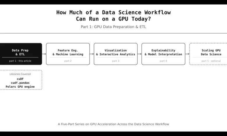
This article embarks on a comprehensive exploration of this evolving landscape. By systematically examining each stage of a typical machine learning pipeline, we will identify where GPU acceleration is currently available, assess the practical implications of its integration, and evaluate the remaining scenarios where CPUs might still hold an advantage. Our initial focus will be on the foundational stages of tabular data processing and the critical data preparation tasks that form the bedrock of many day-to-day data science endeavors.

Dataset and Codebase for Analysis

To provide a tangible and practical demonstration, this analysis will utilize the extensive NYC Yellow Taxi Trip Records dataset. This comprehensive dataset, made available under a Creative Commons license, chronicles millions of taxi journeys across New York City. It contains rich information, including pickup and drop-off coordinates, trip distances, passenger counts, fare details, and precise timestamps. For the purpose of this exploration, we will be working with the data from the first three months of a recent year, which collectively comprises approximately 9 to 10 million records. This substantial volume of data is representative of the scale at which performance bottlenecks can emerge.

The accompanying code examples have been streamlined to maintain focus on the core concepts. Boilerplate code and certain lengthy snippets have been omitted for clarity. The complete, runnable code, allowing for replication and further experimentation, is available on GitHub for public access.

Accelerating Pandas Workflows on the GPU

For data scientists whose existing pipelines are built upon the widely adopted Pandas library, there are two primary avenues for leveraging GPU acceleration: adopting GPU-native libraries with similar APIs or utilizing compatibility layers that enable existing Pandas code to run on the GPU.

1. Building GPU-Native Workflows with the cuDF API

For new projects or when undertaking a significant refactoring, adopting cuDF offers a direct path to GPU-accelerated tabular data manipulation. cuDF is a core component of RAPIDS, NVIDIA’s open-source suite of libraries designed to accelerate data science and analytics tasks using the power of GPUs.

cuDF provides a Python DataFrame API that is remarkably similar to Pandas. This design choice significantly lowers the barrier to entry for experienced Pandas users. The fundamental difference lies in where these operations are executed: cuDF processes data directly on the GPU, leveraging its parallel processing capabilities. While cuDF aims for high API compatibility with Pandas, it’s important to note that it is not a complete one-to-one replacement. Some nuanced behaviors or less common operations might differ.

Installation and Setup:

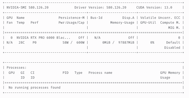
For users of Google Colab, cuDF is often pre-installed and readily available within the GPU runtime environment. For other environments, installation involves selecting a cuDF package that aligns with the installed CUDA version. The CUDA version can be readily identified by executing the !nvidia-smi command in a terminal or notebook.

!nvidia-smi

For instance, if the system reports CUDA version 13.x, the appropriate cuDF package would be installed using:

pip install cudf-cu13

A comprehensive list of installation options and supported CUDA versions can be found in the official cuDF installation guide.

Loading Data into cuDF DataFrames:

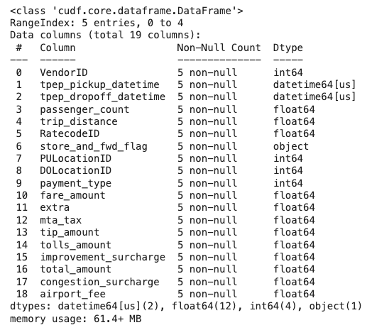
The process of loading data into a cuDF DataFrame mirrors that of Pandas. Typically, one simply replaces Pandas’ read_* functions with their cuDF counterparts. For example, reading a Parquet file:

import cudf

taxi_url = 'https://d37ci6vzurychx.cloudfront.net/trip-data/yellow_tripdata_2023-01.parquet'

df_gpu = cudf.read_parquet(taxi_url)
df_gpu.info()

Once data resides in GPU memory, subsequent DataFrame operations are automatically executed on the GPU, unlocking significant performance gains.

Working with cuDF:

cuDF supports a vast majority of the operations familiar to Pandas users. Key operations include:

• Column Selection:

  trips = df_gpu[ [ "PULocationID", "DOLocationID", "fare_amount", "trip_distance", "tip_amount", ] ]

• Row Filtering:

  high_fare = trips[trips["fare_amount"] > 20]

• Creating New Columns:

  trips["tip_percentage"] = ( trips["tip_amount"] / trips["fare_amount"] * 100 )

• Summary Statistics:

  trips.describe()

Seamless Transition Between Pandas and cuDF:

Many existing data science workflows rely on libraries that are strictly compatible with Pandas DataFrames. cuDF facilitates a smooth transition by allowing data to be moved between CPU and GPU memory as needed.

• Converting Pandas to cuDF:

  df_gpu = cudf.from_pandas(df_cpu)
  print(type(df_gpu_converted))
  # Output: <class 'cudf.core.dataframe.DataFrame'>

• Converting cuDF to Pandas:

  df_cpu = df_gpu.to_pandas()
  print(type(df_cpu_converted))
  # Output: <class 'pandas.core.frame.DataFrame'>

  These conversion capabilities are invaluable for migrating existing Pandas-based workflows to harness GPU acceleration or for integrating GPU-processed data into downstream libraries that only support Pandas.

Performance Benchmarking: Pandas vs. cuDF

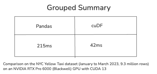
To empirically demonstrate the performance benefits, let’s compare the execution of identical analyses using both Pandas and cuDF. We will group taxi trips by their pickup location and compute aggregate statistics: total fare amount, average trip distance, and the total number of trips.

def summarize_trips(df):
    return (
        df.groupby("PULocationID")
          .agg(
              
                  "fare_amount": "sum",
                  "trip_distance": "mean",
                  "passenger_count": "count",
              
          )
          .sort_values("fare_amount", ascending=False)
    )

# Assuming df_cpu is a Pandas DataFrame and df_gpu is a cuDF DataFrame

%time summary_pd = summarize_trips(df_cpu)
%time summary_gpu = summarize_trips(df_gpu)

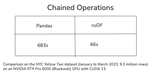
Real-world data processing rarely involves isolated operations. It typically entails a series of chained DataFrame manipulations. As a more realistic benchmark, let’s determine the most frequent drop-off location for each unique pickup location.

def run_chain(df):
    return (
        df[["PULocationID", "DOLocationID"]]
        .value_counts()
        .reset_index(name="count")
        .sort_values(
            ["PULocationID", "count"],
            ascending=[True, False],
        )
        .groupby("PULocationID")
        .head(1)
        .reset_index(drop=True)
    )

%time result_pd = run_chain(df_cpu)
%time result_gpu = run_chain(df_gpu)

Benchmarking Heavy Aggregations

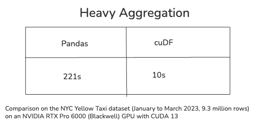
Groupby aggregations represent a cornerstone of analytical pipelines and are exceptionally well-suited for GPU acceleration due to their inherent computational intensity. Let’s benchmark a complex grouped aggregation across multiple columns.

def aggregate(df):
    return (
        df.groupby("PULocationID")
          .agg(
              
                  "fare_amount": "sum",
                  "trip_distance": "sum",
                  "passenger_count": "count",
              
          )
    )

%time agg_pd = aggregate(df_cpu)
%time agg_gpu = aggregate(df_gpu)

Even with the current dataset size, the benchmarks reveal a substantial speedup. For larger datasets, these aggregation-intensive workloads stand to benefit even more dramatically from the parallel processing capabilities of GPUs.

2. Accelerating Existing Pandas Code with cudf.pandas

A frequent question from data scientists is the feasibility of speeding up existing Pandas code without extensive rewriting. While the native cuDF API is ideal for new projects, many established data science workflows are deeply integrated with Pandas. Recognizing this, the RAPIDS ecosystem offers cudf.pandas, an accelerator mode within cuDF that allows existing Pandas code to run on the GPU with virtually no modifications.

Enabling the Accelerator:

To activate GPU acceleration within a notebook environment, the cudf.pandas extension must be loaded before the Pandas library is imported.

%load_ext cudf.pandas
import pandas as pd

For Python scripts, GPU acceleration can be enabled by executing the script via the cudf.pandas module:

python -m cudf.pandas script.py

Seamless Execution with Familiar Pandas Code:

The beauty of cudf.pandas lies in its transparency. We can reuse the exact same data and code snippets from the previous section. The sole addition is the %load_ext cudf.pandas directive, which seamlessly switches the underlying execution engine.

%load_ext cudf.pandas
import pandas as pd

taxi_url = 'https://d37ci6vzurychx.cloudfront.net/trip-data/yellow_tripdata_2023-01.parquet'

df = pd.read_parquet(taxi_url)

summary = (
    df.groupby("PULocationID")
      .agg(
          
              "fare_amount": "sum",
              "trip_distance": "mean",
              "passenger_count": "count",
          
      )
      .sort_values("fare_amount", ascending=False)
)

summary

To confirm that cudf.pandas is active, one can inspect the Pandas module:

print(pd)
# Output: <module 'pandas' (ModuleAccelerator(fast=cudf, slow=pandas))&gt;

Under the hood, cudf.pandas attempts to execute every Pandas operation using cuDF. If a particular operation is not yet supported by cuDF, it gracefully falls back to the standard CPU-based Pandas implementation.

Profiling GPU and CPU Execution:

To gain insight into which operations are being accelerated and which are falling back to the CPU, cudf.pandas includes a built-in profiler.

%%cudf.pandas.profile
summary = (
    df.groupby("payment_type")
      .fare_amount.mean()
)

Upon completion of the cell, the profiler generates a detailed report, clearly delineating GPU-accelerated operations and any CPU fallbacks.

For a more granular analysis, the %%cudf.pandas.line_profile magic command provides a line-by-line breakdown of execution time spent on both the GPU and CPU.

%%cudf.pandas.line_profile
summary = (
    df.groupby("payment_type")
      .fare_amount.mean()
)

Interoperability with Third-Party Libraries:

A significant advantage of cudf.pandas is its adherence to the Pandas API. This means that many libraries that seamlessly integrate with Pandas will continue to function without modification. Data processed on the GPU can be directly passed to visualization libraries like Plotly Express, for instance, without requiring any changes to the downstream visualization code.

import plotly.express as px

top10 = summary.head(10).reset_index()

fig = px.bar(
    top10,
    x="PULocationID",
    y="fare_amount",
    title="Top 10 Pickup Locations by Total Fare",
    labels=
        "PULocationID": "Pickup Location ID",
        "fare_amount": "Total Fare",
    ,
)

fig.show()

This process generates the same interactive visualizations as would be produced with standard Pandas, but with the added benefit of significantly accelerated data processing. The preservation of downstream code ensures a remarkably smooth integration of GPU acceleration into existing notebooks and analytical pipelines, without disrupting established visualization workflows.

3. Harnessing the Polars GPU Engine

Polars, already renowned for its high-performance DataFrame engine and efficient Lazy API, offers further acceleration through its GPU engine, powered by cuDF. This capability is particularly impactful for users working with very large datasets. Similar to cudf.pandas, the Polars GPU engine enables acceleration of existing workflows with minimal code alterations.

When a lazy query is executed in Polars, the engine first constructs an optimized query plan. If the operations within this plan are supported by the GPU, they are processed using cuDF. Otherwise, Polars seamlessly transitions to its established CPU-based engine.

Installation:

The most straightforward method to install the GPU engine for Polars is by using the optional polars[gpu] package, which automatically manages the installation of necessary RAPIDS dependencies.

pip install "polars[gpu]"

# Alternatively, for direct cuDF-backed Polars engine installation with CUDA 12:
pip install -q polars cudf-polars-cu12 --extra-index-url=https://pypi.nvidia.

Enabling GPU Acceleration in Polars:

We will employ the same NYC taxi dataset and replicate the analytical tasks performed in previous sections. The key difference lies in specifying engine="gpu" when calling the collect() method, directing Polars to utilize the GPU engine.

import polars as pl

taxi_url = "https://d37ci6vzurychx.cloudfront.net/trip-data/yellow_tripdata_2023-01.parquet"

query = (
    pl.scan_parquet(taxi_url)
      .group_by("PULocationID")
      .agg(
          fare_amount=pl.col("fare_amount").sum(),
          trip_distance=pl.col("trip_distance").mean(),
          trip_count=pl.len(),
      )
      .sort("fare_amount", descending=True)
)

summary = query.collect(engine="gpu")
summary.head()

The query construction remains identical to a standard Polars LazyFrame workflow. The sole modification is the engine="gpu" argument in collect(), instructing Polars to leverage the GPU engine where operation support exists. Crucially, if the query incorporates unsupported operations, Polars automatically reverts to its CPU engine.

Verifying GPU Execution:

To confirm whether a query has been executed on the GPU, verbose mode can be enabled prior to calling collect(). If a query cannot be processed on the GPU, Polars will issue a PerformanceWarning detailing the reason for the fallback to the CPU. For stricter control, automatic fallback can be disabled by passing pl.GPUEngine(raise_on_fail=True) to collect(), which will trigger an error if the query is not fully supported on the GPU.

# Assuming df_lazy is a Polars LazyFrame

unsupported_gpu_operation = (
    df_lazy
    .select(
        pl.col("fare_amount")
        .map_elements(lambda fare: fare * 1.1, return_dtype=pl.Float64)
        .alias("fare_with_markup")
    )
    .head(10)
)

with pl.Config() as cfg:
    cfg.set_verbose(True)
    fallback_result = unsupported_gpu_operation.collect(engine="gpu")

print(fallback_result)

In the example above, the use of map_elements() with a Python lambda function is intentionally demonstrated. Since Python functions are not inherently supported by the Polars GPU engine, this specific query necessitates a fallback to the CPU.

Scaling to Multiple GPUs:

The examples presented thus far utilize a single GPU. For scenarios involving exceptionally large datasets or when multiple GPUs are available, scaling can be achieved with a minor modification using the RayEngine.

from cudf_polars.engine.ray import RayEngine

# Assuming 'query' is the Polars LazyFrame defined earlier

with RayEngine() as engine:
    summary = query.collect(engine=engine)

The RayEngine automatically leverages all GPUs accessible to the process, enabling a single lazy query to scale efficiently from one GPU to multiple. For a deeper understanding of how the Polars GPU engine scales across multiple GPUs, Benjamin Zaitlen’s insightful blog post offers a comprehensive walkthrough of the underlying concepts and includes illustrative performance examples.

Conclusion: A New Era for Tabular Data Analysis

The benchmarks and practical experiments consistently highlight that GPUs are most effective for large-scale, data-intensive operations. These include complex filtering, joins, aggregations, and sorting tasks. For smaller datasets, the overhead associated with transferring data to the GPU can sometimes negate the performance benefits, making CPUs a competitive or even superior choice.

The advent of libraries like cuDF and the integration within frameworks like cudf.pandas and the Polars GPU engine have dramatically lowered the barrier to GPU acceleration. Data scientists are no longer faced with the daunting prospect of rewriting entire codebases to achieve performance gains. Instead, they can strategically switch between GPU and CPU execution, optimizing for the specific demands of their workloads. This newfound flexibility translates directly into reduced waiting times for query execution and more time dedicated to critical analytical tasks, ultimately accelerating the pace of discovery and innovation in data science.

The subsequent article in this series will venture beyond data preparation and delve into the realm of GPU acceleration for machine learning libraries. We will investigate the extent to which model training can be expedited and the degree of code modification required to achieve these speedups.

Note: All images in this work are by the author unless otherwise stated or attributed.